Calculating liquidity

Trading is not possible without liquidity, and to make our first swap we need to put some liquidity into the pool contract. Here’s what we need to know to add liquidity to the pool contract:

1. A price range. As a liquidity provider, we want to provide liquidity at a specific price range, and it’ll only be used in this range.
2. Amount of liquidity, which is the amounts of two tokens. We’ll need to transfer these amounts to the pool contract.

Here, we’re going to calculate these manually, but, in a later chapter, a contract will do this for us. Let’s begin with a price range.

Price Range Calculation

Recall that, in Uniswap V3, the entire price range is demarcated into ticks: each tick corresponds to a price and has an index. In our first pool implementation, we’re going to buy ETH for USDC at the price of $5000 per 1 ETH. Buying ETH will remove some amount of it from the pool and will push the price slightly above $5000. We want to provide liquidity at a range that includes this price. And we want to be sure that the final price will stay within this range (we’ll do multi-range swaps in a later milestone).

We’ll need to find three ticks:

1. The current tick will correspond to the current price (5000 USDC for 1 ETH).
2. The lower and upper bounds of the price range we’re providing liquidity into. Let the lower price be $4545 and the upper price be $5500.

From the theoretical introduction, we know that:

$$\sqrt{P}=\sqrt{\frac{y}{x}}$$

Since we’ve agreed to use ETH as the $x$ reserve and USDC as the $y$ reserve, the prices at each of the ticks are:

$$\sqrt{P_c}=\sqrt{\frac{5000}{1}}=\sqrt{5000}\approx 70.71$$

$$\sqrt{P_l}=\sqrt{\frac{4545}{1}}\approx 67.42$$

$$\sqrt{P_u}=\sqrt{\frac{5500}{1}}\approx 74.16$$

Where $P_c$ is the current price, $P_l$ is the lower bound of the range, and $P_u$ is the upper bound of the range.

Now, we can find corresponding ticks. We know that prices and ticks are connected via this formula:

$$\sqrt{P(i)}=1.0001^{\frac{i}{2}}$$

Thus, we can find tick $i$ via:

$$i=lo{g}_{\sqrt{1.0001}}\sqrt{P(i)}$$

The square roots in this formula cancel out, but since we’re working with $\sqrt{p}$ we need to preserve them.

Let’s find the ticks:

1. Current tick: $i_c=lo{g}_{\sqrt{1.0001}}70.71=85176$
2. Lower tick: $i_l=lo{g}_{\sqrt{1.0001}}67.42=84222$
3. Upper tick: $i_u=lo{g}_{\sqrt{1.0001}}74.16=86129$

To calculate these, I used Python:

import math

def price_to_tick(p):
    return math.floor(math.log(p, 1.0001))

price_to_tick(5000)
> 85176

That’s it for price range calculation!

Last thing to note here is that Uniswap uses Q64.96 number to store $\sqrt{P}$. This is a fixed-point number that has 64 bits for the integer part and 96 bits for the fractional part. In our above calculations, prices are floating point numbers: 70.71, 67.42, and 74.16. We need to convert them to Q64.96. Luckily, this is simple: we need to multiply the numbers by $2^{96}$ (Q-number is a binary fixed-point number, so we need to multiply our decimals numbers by the base of Q64.96, which is $2^{96}$). We’ll get:

$$\sqrt{P_c}=5602277097478614198912276234240$$

$$\sqrt{P_l}=5314786713428871004159001755648$$

$$\sqrt{P_u}=5875717789736564987741329162240$$

In Python:

q96 = 2**96
def price_to_sqrtp(p):
    return int(math.sqrt(p) * q96)

price_to_sqrtp(5000)
> 5602277097478614198912276234240

Notice that we’re multiplying before converting to an integer. Otherwise, we’ll lose precision.

Token Amounts Calculation

The next step is to decide how many tokens we want to deposit into the pool. The answer is as many as we want. The amounts are not strictly defined, we can deposit as much as it is enough to buy a small amount of ETH without making the current price leave the price range we put liquidity into. During development and testing we’ll be able to mint any amount of tokens, so getting the amounts we want is not a problem.

For our first swap, let’s deposit 1 ETH and 5000 USDC.

Recall that the proportion of current pool reserves tells the current spot price. So if we want to put more tokens into the pool and keep the same price, the amounts must be proportional, e.g.: 2 ETH and 10,000 USDC; 10 ETH and 50,000 USDC, etc.

Liquidity Amount Calculation

Next, we need to calculate $L$ based on the amounts we’ll deposit. This is a tricky part, so hold tight!

From the theoretical introduction, you remember that: $$L=\sqrt{xy}$$

However, this formula is for the infinite curve 🙂 But we want to put liquidity into a limited price range, which is just a segment of that infinite curve. We need to calculate $L$ specifically for the price range we’re going to deposit liquidity into. We need some more advanced calculations.

To calculate $L$ for a price range, let’s look at one interesting fact we have discussed earlier: price ranges can be depleted. It’s possible to buy the entire amount of one token from a price range and leave the pool with only the other token.

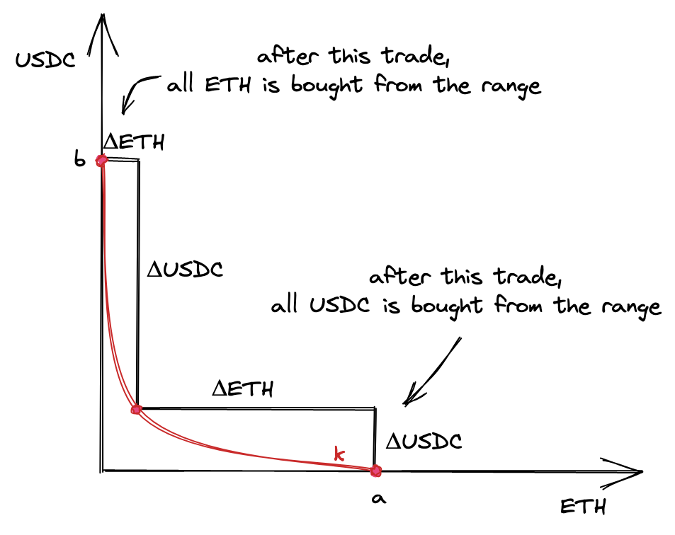
At the points $a$ and $b$, there’s only one token in the range: ETH at the point $a$ and USDC at the point $b$.

That being said, we want to find an $L$ that will allow the price to move to either of the points. We want enough liquidity for the price to reach either of the boundaries of a price range. Thus, we want $L$ to be calculated based on the maximum amounts of $\Delta x$ and $\Delta y$.

Now, let’s see what the prices are at the edges. When ETH is bought from a pool, the price is growing; when USDC is bought, the price is falling. Recall that the price is $\frac{y}{x}$. So, at point $a$, the price is the lowest of the range; at point $b$, the price is the highest.

In fact, prices are not defined at these points because there’s only one reserve in the pool, but what we need to understand here is that the price around the point $b$ is higher than the start price, and the price at the point $a$ is lower than the start price.

Now, break the curve from the image above into two segments: one to the left of the start point and one to the right of the start point. We’re going to calculate two $L$’s, one for each of the segments. Why? Because each of the two tokens of a pool contributes to either of the segments: the left segment is made entirely of token $x$, and the right segment is made entirely of token $y$. This comes from the fact that, during swapping, the price moves in either direction: it’s either growing or falling. For the price to move, only either of the tokens is needed:

1. when the price is growing, only token $x$ is needed for the swap (we’re buying token $x$, so we want to take only token $x$ from the pool);
2. when the price is falling, only token $y$ is needed for the swap.

Thus, the liquidity in the segment of the curve to the left of the current price consists only of token $x$ and is calculated only from the amount of token $x$ provided. Similarly, the liquidity in the segment of the curve to the right of the current price consists only of token $y$ and is calculated only from the amount of token $y$ provided.

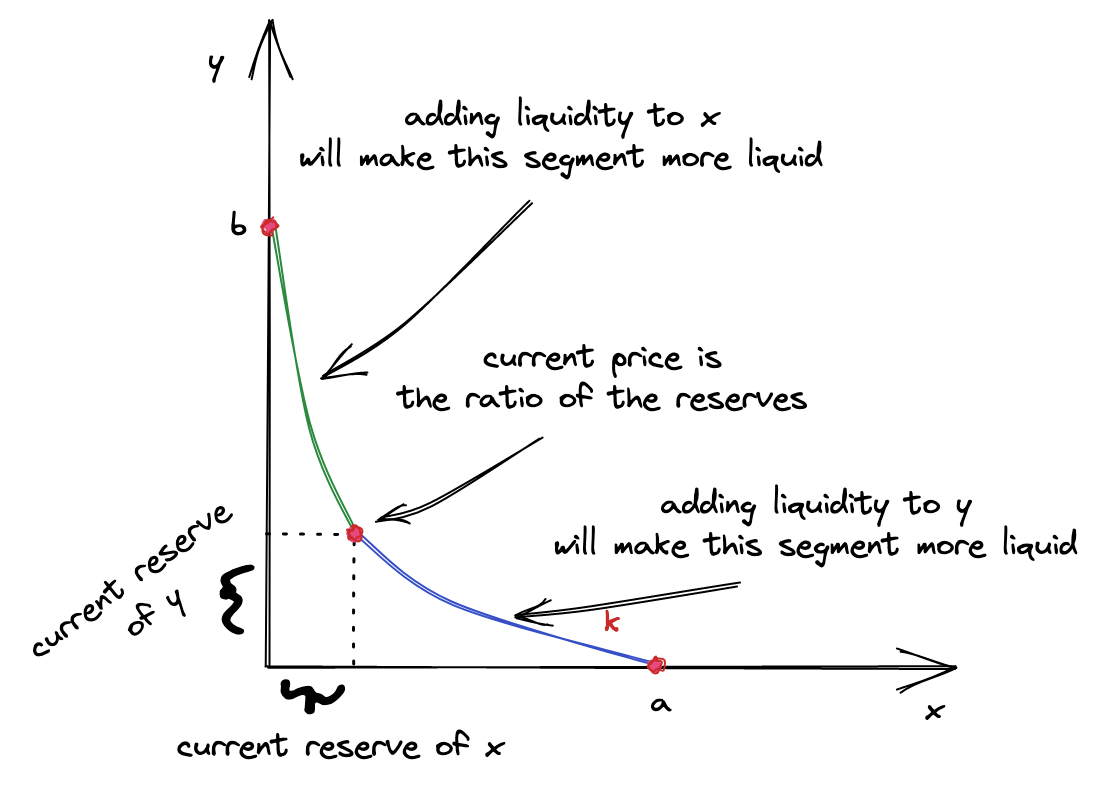
This is why, when providing liquidity, we calculate two $L$’s and pick one of them. Which one? The smaller one. Why? Because the bigger one already includes the smaller one! We want the new liquidity to be distributed evenly along the curve, thus we want to add the same $L$ to the left and to the right of the current price. If we pick the bigger one, the user would need to provide more liquidity to compensate for the shortage in the smaller one. This is doable, of course, but this would make the smart contract more complex.

What happens with the remainder of the bigger $L$? Well, nothing. After picking the smaller $L$ we can simply convert it to a smaller amount of the token that resulted in the bigger $L$–this will adjust it down. After that, we’ll have token amounts that will result in the same $L$.

The final detail I need to focus your attention on here is: new liquidity must not change the current price. That is, it must be proportional to the current proportion of the reserves. And this is why the two $L$’s can be different–when the proportion is not preserved. And we pick the small $L$ to reestablish the proportion.

I hope this will make more sense after we implement this in code! Now, let’s look at the formulas.

Let’s recall how $\Delta x$ and $\Delta y$ are calculated:

$$\Delta x=\Delta \frac{1}{\sqrt{P}}L$$ $$\Delta y=\Delta \sqrt{P}L$$

We can expand these formulas by replacing the delta P’s with actual prices (we know them from the above):

$$\Delta x=(\frac{1}{\sqrt{P_c}}-\frac{1}{\sqrt{P_b}})L$$ $$\Delta y=(\sqrt{P_c}-\sqrt{P_a})L$$

$P_a$ is the price at the point $a$, $P_b$ is the price at the point $b$, and $P_c$ is the current price (see the above chart). Notice that, since the price is calculated as $\frac{y}{x}$ (i.e. it’s the price of $x$ in terms of $y$), the price at point $b$ is higher than the current price and the price at $a$. The price at $a$ is the lowest of the three.

Let’s find the $L$ from the first formula:

$$\Delta x=(\frac{1}{\sqrt{P_c}}-\frac{1}{\sqrt{P_b}})L$$ $$\Delta x=\frac{L}{\sqrt{P_c}}-\frac{L}{\sqrt{P_b}}$$ $$\Delta x=\frac{L(\sqrt{P_b}-\sqrt{P_c})}{\sqrt{P_b}\sqrt{P_c}}$$ $$L=\Delta x\frac{\sqrt{P_b}\sqrt{P_c}}{\sqrt{P_b}-\sqrt{P_c}}$$

And from the second formula: $$\Delta y=(\sqrt{P_c}-\sqrt{P_a})L$$ $$L=\frac{\Delta y}{\sqrt{P_c}-\sqrt{P_a}}$$

So, these are our two $L$’s, one for each of the segments:

$$L=\Delta x\frac{\sqrt{P_b}\sqrt{P_c}}{\sqrt{P_b}-\sqrt{P_c}}$$ $$L=\frac{\Delta y}{\sqrt{P_c}-\sqrt{P_a}}$$

Now, let’s plug the prices we calculated earlier into them:

$$L=\Delta x\frac{\sqrt{P_b}\sqrt{P_c}}{\sqrt{P_b}-\sqrt{P_c}}=1ETH\ast \frac{5875\dots \ast 5602\dots }{5875\dots -5602\dots }$$

After converting to Q64.96, we get:

$$L=1519437308014769733632$$

And for the other $L$: $$L=\frac{\Delta y}{\sqrt{P_c}-\sqrt{P_a}}=\frac{5000USDC}{5602\dots -5314\dots }$$ $$L=1517882343751509868544$$

Of these two, we’ll pick the smaller one.

In Python:

sqrtp_low = price_to_sqrtp(4545)
sqrtp_cur = price_to_sqrtp(5000)
sqrtp_upp = price_to_sqrtp(5500)

def liquidity0(amount, pa, pb):
    if pa > pb:
        pa, pb = pb, pa
    return (amount * (pa * pb) / q96) / (pb - pa)

def liquidity1(amount, pa, pb):
    if pa > pb:
        pa, pb = pb, pa
    return amount * q96 / (pb - pa)

eth = 10**18
amount_eth = 1 * eth
amount_usdc = 5000 * eth

liq0 = liquidity0(amount_eth, sqrtp_cur, sqrtp_upp)
liq1 = liquidity1(amount_usdc, sqrtp_cur, sqrtp_low)
liq = int(min(liq0, liq1))
> 1517882343751509868544

Token Amounts Calculation, Again

Since we choose the amounts we’re going to deposit, the amounts can be wrong. We cannot deposit any amounts at any price range; the liquidity amount needs to be distributed evenly along the curve of the price range we’re depositing into. Thus, even though users choose amounts, the contract needs to re-calculate them, and actual amounts will be slightly different (at least because of rounding).

Luckily, we already know the formulas:

$$\Delta x=\frac{L(\sqrt{P_b}-\sqrt{P_c})}{\sqrt{P_b}\sqrt{P_c}}$$ $$\Delta y=L(\sqrt{P_c}-\sqrt{P_a})$$

In Python:

def calc_amount0(liq, pa, pb):
    if pa > pb:
        pa, pb = pb, pa
    return int(liq * q96 * (pb - pa) / pa / pb)


def calc_amount1(liq, pa, pb):
    if pa > pb:
        pa, pb = pb, pa
    return int(liq * (pb - pa) / q96)

amount0 = calc_amount0(liq, sqrtp_upp, sqrtp_cur)
amount1 = calc_amount1(liq, sqrtp_low, sqrtp_cur)
(amount0, amount1)
> (998976618347425408, 5000000000000000000000)

As you can see, the numbers are close to the amounts we want to provide, but ETH is slightly smaller.

Hint: use cast --from-wei AMOUNT to convert from wei to ether, e.g.:
cast --from-wei 998976618347425280 will give you 0.998976618347425280.