Introduction to Uniswap V3

This chapter retells the whitepaper of Uniswap V3. Again, it’s totally ok if you don’t understand all the concepts. They will be clearer when converted to code.

To better understand the innovations Uniswap V3 brings, let’s first look at the imperfections of Uniswap V2.

Uniswap V2 is a general exchange that implements one AMM algorithm. However, not all trading pairs are equal. Pairs can be grouped by price volatility:

1. Tokens with medium and high price volatility. This group includes most tokens since most tokens don’t have their prices pegged to something and are subject to market fluctuations.
2. Tokens with low volatility. This group includes pegged tokens, mainly stablecoins: USDC/USDT, USDC/DAI, USDT/DAI, etc. Also: ETH/stETH, ETH/rETH (variants of wrapped ETH).

These groups require different, let’s call them, pool configurations. The main difference is that pegged tokens require high liquidity to reduce the demand effect (we learned about it in the previous chapter) on big trades. The prices of USDC and USDT must stay close to 1, no matter how big the number of tokens we want to buy and sell. Since Uniswap V2’s general AMM algorithm is not very well suited for stablecoin trading, alternative AMMs (mainly Curve) were more popular for stablecoin trading.

What caused this problem is that liquidity in Uniswap V2 pools is distributed infinitely–pool liquidity allows trades at any price, from 0 to infinity:

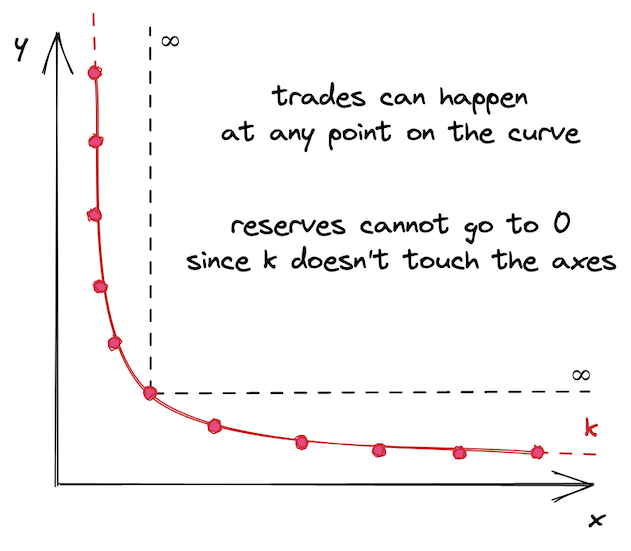
This might not seem like a bad thing, but this makes capital inefficient. Historical prices of an asset stay within some defined range, whether it’s narrow or wide. For example, the historical price range of ETH is from $0.75to$4,800 (according to CoinMarketCap). Today (June 2022, 1 ETH costs $1,800), no one would buy 1 ether at $5000, so it makes no sense to provide liquidity at this price. Thus, it doesn’t make sense to provide liquidity in a price range that’s far away from the current price or that will never be reached.

However, we all believe in ETH reaching $10,000 one day.

Concentrated Liquidity

Uniswap V3 introduces concentrated liquidity: liquidity providers can now choose the price range they want to provide liquidity into. This improves capital efficiency by allowing to put more liquidity into a narrow price range, which makes Uniswap more diverse: it can now have pools configured for pairs with different volatility. This is how V3 improves V2.

In a nutshell, a Uniswap V3 pair is many small Uniswap V2 pairs. The main difference between V2 and V3 is that, in V3, there are many price ranges in one pair. And each of these shorter price ranges has finite reserves. The entire price range from 0 to infinite is split into shorter price ranges, with each of them having its own amount of liquidity. But, what’s crucial is that within that shorter price range, it works exactly as Uniswap V2. This is why I say that a V3 pair is many small V2 pairs.

Now, let’s try to visualize it. What we’re saying is that we don’t want the curve to be infinite. We cut it at the points $a$ and $b$ and say that these are the boundaries of the curve. Moreover, we shift the curve so the boundaries lay on the axes. This is what we get:

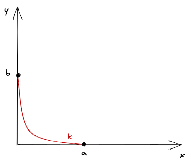
It looks lonely, doesn’t it? This is why there are many price ranges in Uniswap V3–so they don’t feel lonely 🙂

As we saw in the previous chapter, buying or selling tokens moves the price along the curve. A price range limits the movement of the price. When the price moves to either of the points, the pool becomes depleted: one of the token reserves will be 0, and buying this token won’t be possible.

On the chart above, let’s assume that the start price is at the middle of the curve. To get to the point $a$, we need to buy all available $y$ and maximize $x$ in the range; to get to the point $b$, we need to buy all available $x$ and maximize $y$ in the range. At these points, there’s only one token in the range!

Fun fact: this allows using Uniswap V3 price ranges as limit orders!

What happens when the current price range gets depleted during a trade? The price slips into the next price range. If the next price range doesn’t exist, the trade ends up partially fulfilled-we’ll see how this works later in the book.

This is how liquidity is spread in the USDC/ETH pool in production:

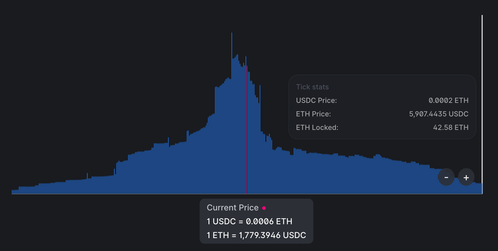
You can see that there’s a lot of liquidity around the current price but the further away from it the less liquidity there is–this is because liquidity providers strive to have higher efficiency of their capital. Also, the whole range is not infinite, its upper boundary is shown in the image.

The Mathematics of Uniswap V3

Mathematically, Uniswap V3 is based on V2: it uses the same formulas, but they’re… let’s call it augmented.

To handle transitioning between price ranges, simplify liquidity management, and avoid rounding errors, Uniswap V3 uses these new concepts:

$$L=\sqrt{xy}$$

$$\sqrt{P}=\sqrt{\frac{y}{x}}$$

$L$ is the amount of liquidity. Liquidity in a pool is the combination of token reserves (that is, two numbers). We know that their product is $k$, and we can use this to derive the measure of liquidity, which is $\sqrt{xy}$–a number that, when multiplied by itself, equals $k$. $L$ is the geometric mean of $x$ and $y$.

$y/x$ is the price of token 0 in terms of 1. Since token prices in a pool are reciprocals of each other, we can use only one of them in calculations (and by convention Uniswap V3 uses $y/x$). The price of token 1 in terms of token 0 is simply $\frac{1}{y/x}=\frac{x}{y}$. Similarly, $\frac{1}{\sqrt{P}}=\frac{1}{\sqrt{y/x}}=\sqrt{\frac{x}{y}}$.

Why using $\sqrt{p}$ instead of $p$? There are two reasons:

1. Square root calculation is not precise and causes rounding errors. Thus, it’s easier to store the square root without calculating it in the contracts (we will not store $x$ and $y$ in the contracts).

2. $\sqrt{P}$ has an interesting connection to $L$: $L$ is also the relation between the change in output amount and the change in $\sqrt{P}$.

   $$L=\frac{\Delta y}{\Delta \sqrt{P}}$$

Proof: $$L=\frac{\Delta y}{\Delta \sqrt{P}}$$ $$\sqrt{xy}=\frac{y_1-y_0}{\sqrt{P_1}-\sqrt{P_0}}$$ $$\sqrt{xy}(\sqrt{P_1}-\sqrt{P_0})=y_1-y_0$$ $$\sqrt{xy}(\sqrt{\frac{y_1}{x_1}}-\sqrt{\frac{y_0}{x_0}})=y_1-y_0$$ $$\text{Since }\sqrt{x_1{y}_1}=\sqrt{x_0{y}_0}=\sqrt{xy}=L,$$ $$\sqrt{\frac{x_1{y}_1{y}_1}{x_1}}-\sqrt{\frac{x_0{y}_0{y}_0}{x_0}}=y_1-y_0$$ $$\sqrt{y_1^2}-\sqrt{y_0^2}=y_1-y_0$$ $$y_1-y_0=y_1-y_0$$

Pricing

Again, we don’t need to calculate actual prices–we can calculate the output amount right away. Also, since we’re not going to track and store $x$ and $y$, our calculation will be based only on $L$ and $\sqrt{P}$.

From the above formula, we can find $\Delta y$:

$$\Delta y=\Delta \sqrt{P}L$$

See the third step in the proof above.

As we discussed above, prices in a pool are reciprocals of each other. Thus, $\Delta x$ is:

$$\Delta x=\Delta \frac{1}{\sqrt{P}}L$$

$L$ and $\sqrt{P}$ allow us to not store and update pool reserves. Also, we don’t need to calculate $\sqrt{P}$ each time because we can always find $\Delta \sqrt{P}$ and its reciprocal.

Ticks

As we learned in this chapter, the infinite price range of V2 is split into shorter price ranges in V3. Each of these shorter price ranges is limited by boundaries–upper and lower points. To track the coordinates of these boundaries, Uniswap V3 uses ticks.

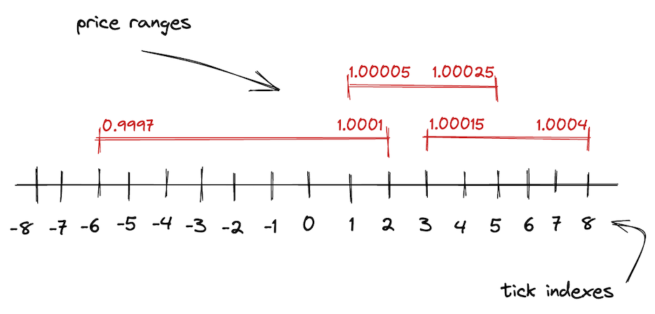
In V3, the entire price range is demarcated by evenly distributed discrete ticks. Each tick has an index and corresponds to a certain price:

$$p(i)=1.0001^i$$

Where $p(i)$ is the price at tick $i$. Taking powers of 1.0001 has a desirable property: the difference between two adjacent ticks is 0.01% or 1 basis point.

Basis point (1/100th of 1%, or 0.01%, or 0.0001) is a unit of measure of percentages in finance. You could’ve heard about the basis point when central banks announced changes in interest rates.

As we discussed above, Uniswap V3 stores $\sqrt{P}$, not $P$. Thus, the formula is in fact:

$$\sqrt{p(i)}={\sqrt{1.0001}}^i=1.0001^{\frac{i}{2}}$$

So, we get values like: $\sqrt{p(0)}=1$, $\sqrt{p(1)}=\sqrt{1.0001}\approx 1.00005$, $\sqrt{p(-1)}\approx 0.99995$.

Ticks are integers that can be positive and negative and, of course, they’re not infinite. Uniswap V3 stores $\sqrt{P}$ as a fixed point Q64.96 number, which is a rational number that uses 64 bits for the integer part and 96 bits for the fractional part. Thus, prices (equal to the square of $\sqrt{P}$) are within the range: $[2^{-128},2^{128}]$. And ticks are within the range:

$$[lo{g}_{1.0001}{2}^{-128},lo{g}_{1.0001}{2}^{128}]=[-887272,887272]$$

For deeper dive into the math of Uniswap V3, I cannot but recommend this technical note by Atis Elsts.